Several outlooks on differential equations

In math as in life, the same object of study can be looked upon from multiple perspectives. Each perspective offers a different insight into a problem, and often the same problem can be very difficult from one perspective, yet clear from another.

In this post I will discuss three different ways to think about differential equations.

The algebraic perspective

The algebraic way to think about differential equations is perhaps the most familiar, as at least on first sight it might look similar to the regular equations we encounter in school. Some examples are:

or

where the variable \(x\) stands for an unknown function of a variable \(t\), and \(x'\) is the derivative etc. This presentation suggests that some algebraic manipulations will reveal the answer, again like solving equations in school.

The technique of separation of variables (mentioned in the previous post) belongs to this category. For example, the second example above can be solved by

which only contains algebraic manipulations and calculus. While the algebraic perspective is straightforward, it doesn't tell the whole story, and it might leave us hanging when the equation is (or seems) insoluble.

The geometric perspective

This perspective is very much the focus of the book "Nonlinear Dynamics and Chaos" by Steven Strogatz, at least the part I read so far (which is admittedly not much). Let's consider the equation

It can be solved algebraically using the characteristic polynomial to get two basis solutions \(x_1(t)=\sin t\) and \(x_2(t)=\cos t\), but we will consider a different approach. Let's define a new variable \(v=x'\). This transforms the second-order differential equation to a first-order system of two equations

We can imagine the \((x,v)\) plane.

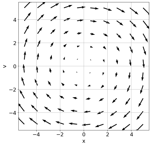
We can think of these equations as defining a vector field over the plane

We usually visualize vector fields by drawing arrows originating from points in the plane, with the size indicating magnitude:

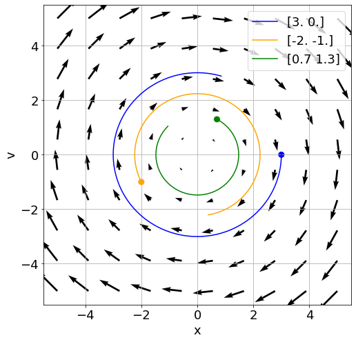
If we imagine a particle starting from some point on the plane, the vector field tells us where it will flow on the next moment. We can further imagine it flowing from moment to moment, and get a trajectory, or a curve, through the plane. Here is a plot of curves from three different starting points, generated using the same process:

Let's call the curve we got \(\phi\). So \(\phi\) is a function mapping time \(t\) to a point on the plane, and from how we "defined" it, the tangent to the curve at each point on the curve \((\phi_x(t),\phi_v(t))\) is the vector field at that point \(f(\phi_x(t),\phi_v(t))\). I claim that \(\phi_x\), the first coordinate of the curve, is a solution to the differential equation:

In fact, any curve that satisfies this property, that the tangent to the curve at a point is equal to the vector field at that point, is a solution to the differential equation. The beauty of this approach is that it is intuitively clear from the picture of the vector field that solutions exist for every initial condition, and how the solution will look like (for example, that it is periodic). We can also read off qualitative properties, like stationary points.

Of course, existence (and uniqueness) of solutions requires a proof, which is not trivial. Still, looking at the picture shows it to be plausible, whereas looking at the differential equation gives us no such clue.

The operator perspective

On this perspective I have little to say, as I still don't know much about it. Still, I find it intriguing, but I warn that this section is more of a "ramble".

The most general definition of differential equation of order \(n\) as an equation

where \(f\) is smooth and a solution is a function \(\phi\) that satisfies this equation

In the case of a linear differential equation then \(f\) is a linear operator, which we can for convenience note as \(L\). If we take the level of abstraction a bit higher, we can think of \(L\) as linear operator on the vector space of smooth functions. For example, we can think of the equation \(x''-x'+x=0\) as defining an operator \(L(\phi)(t)=\phi''(t)-\phi'(t)+\phi(t)\) that maps \(\phi\) to some new function \(\psi\) so defined. Then a solution to the differential equation is simply a function that maps to the zero function!

Now, in linear algebra we talk about the kernel of linear transformations, the set of vectors mapped to the zero vector, and the various cases where it is or is not trivial. To be honest, I don't know how much of that carries over to the case above, since some care is required (for example, the space of smooth functions is infinite-dimensional). Still, something to think about.