"It’s better to do something simple which is real. It’s something you can build on because you know what you’re doing. Whereas, if you try to approximate something very advanced and you don’t know what you’re doing, you can’t build on it." - Bill Evans
Recently I've been trying to brush up on my deep learning practitioner skills, which have atrophied over the last year or so of disuse. Well, not just brush up, but deepen, expand enrich, as what I did in my Masters was really just a part of the work required. I kept trying to approach exciting and ambitious projects only to end up feeling paralysed and overwhelmed, and giving up on them. Luckily I did some honest thinking and acknowledged that my grasp of the practical basics was not strong enough, which meant going back to the woodshed. Also, small projects can act as small wins and box ticks, creating momentum etc.
Today were tackling the IMDB movie sentiment classification database. It contains 50k examples of a binary classification task, deciding whether a movie review is positive or negative. I got the idea from the Claude chatbot, and we will follow Claude's "six-steps plan", each step in its own section.
"Understand the problem and the dataset"
The first step is to download the data from here. Since we're cool, we're gonna use curl and tar. Looking at the extracted folder we see the following structure (reduced to the relevant files)
aclImdb
├── README
├── test
│   ├── neg
│   │   ├── {id}_{rating}.txt
│   │   ├── ...
│   ├── pos
│   │   ├── {id}_{rating}.txt
│   │   └── ...
└── train
    ├── labeledBow.feat
    ├── neg
    │   ├── {id}_{rating}.txt
    │   ├── ...
    └── pos
        ├── {id}_{rating}.txt
        ├── ...
Each text file is a review. The folder determines the label, and we already have a test-train split. Let's look at a review:
cat aclImdb/train/pos/2435_8.txt

I never thought an old cartoon would bring tears to my eyes! When I first purchased Casper & Friends: Spooking About Africa, I so much wanted to see the very first Casper cartoon entitled The Friendly Ghost (1945), But when I saw the next cartoon, There's Good Boos To-Night (1948), It made me break down! I couldn't believe how sad and tragic it was after seeing Casper's fox get killed! I never saw anything like that in the other Casper cartoons! This is the saddest one of all! It was so depressing, I just couldn't watch it again. It's just like seeing Lassie die at the end of a movie. I know it's a classic,But it's too much for us old cartoon fans to handle like me! If I wanted to watch something old and classic, I rather watch something happy and funny! But when I think about this Casper cartoon, I think about my cats!
Wow, almost looks fake. Here's the same id but from the negative folder
cat aclImdb/train/neg/2435_1.txt

I will warn you here: I chose to believe those reviewers who said that this wasn't an action film in the usual sense, rather a psychological drama so you should appreciate it on that basis and you will be alright.<br /><br />I am here to tell you that they were wrong. Completely wrong.<br /><br />Well, no, not completely; it is very disappointing if you are looking for an action flick, they were right about that. But it is also very unsatisfying on all other levels as well.<br /><br />Tom Beringer wasn't too bad, I suppose, no worse than usual; but what possessed them to cast Billy Zane in this? Was it some sort of death wish on the part of the producers? A way to made their film a guaranteed flop? In that case, it worked.<br /><br />If they were actually aiming for success, then why not cast somebody who can act? Oh, and might as well go for a screenwriter who knows how to write. Ah, yes, and a director who knows how to direct.<br /><br />As someone who sat through this mess, actually believing it would shortly redeem itself, I can assure you it never did. Pity, it could've been a good film.
Here we also see some html tags, which we will probably want to filter out. That's a classic example of why it's good to look at the data, since some unexpected thing can always mess with your model.
"Preprocess the data"
Since the dataset is relatively small (couple hundred mb), we can afford to load it in memory.
import os
from pathlib import Path

data = {}
for split in ['train', 'test']:
    data[split] = {}
    for label in ['pos', 'neg']:
        data[split][label] = []
        p = Path(f'aclImdb/{split}/{label}')
        for name in os.listdir(dir):
            with open(dir/name) as f:
                data[split][label].append(f.read())
This snippet will load all the data into a dictionary mirroring the folder structure.
Even though we're still in the preprocessing stage, we already need to start considering our model, because this determines the kind of preprocessing we do. We will take as a baseline a combination of bag-of-words and logistic regression. bag-of-words will produce a vector which we can feed into the logistic regression. Bag-of-words turns a sentence into a vector by counting the number of occurrences of each word, (like the Counter data structure in python's collections, but as a vector). Since we turn it to a vector, we must select some size for the vocabulary, the set of words the model recognizes. We'll consider words to be a space delimited string, and get rid of punctuation. The size of the vocabulary will be determined from the distribution of words in the corpus, or to put it differently, we're going to try to choose a number that's small while still not requiring us to throw away a lot of words.
We also do some preprocessing by turning everything to lower-case and getting rid of punctuations.
import re
from collections import Counter

c = Counter()
for r in data['train']['pos']+data['train']['neg']:
    c.update(re.sub(r'[^a-z\s]', '', r.lower()).split())
The top 10 words in the corpus are then
Counter({'the': 334760,
         'and': 162243,
         'a': 161962,
         'of': 145332,
         'to': 135047,
         'is': 106859,
         'in': 93038,
         'it': 77110,
         'i': 75738,
         ...
Of course, all the most common words are quite generic. We can plot the this on a graph.
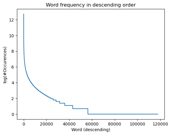
Some thoughts before we move on: - The most common words are actually not useful at all on their own. - We see from the graph that about half the words appear only once. - Since the number of words we take determines the dimensions of the feature vector, we should keep in mind the number of training samples we have (~50k). We want the number of features to be small enough to avoid overfitting. - We can surely reduce the number of words by using better tokenization. For example, in our current scheme a word like "valentine's" turns to "valentines", but the interesting word is really "valentine".
For now, we start with an arbitrary vocab_size of 5000.
vocab_size = 5000
vocab = {k: i for i, k in enumerate(sorted(c, key=c.get, reverse=True)[:vocab_size])}
And we use it to build a feature vector by counting occurrences of words that are in the vocabulary.
def features(review, vocab):
    words = tokenize(review)
    vec = np.zeros(len(vocab))
    for w in words:
        if w in vocab:
            vec[vocab[w]] += 1
    return vec

features("the bear was awesome", vocab)
# array([1., 0., 0., ..., 0., 0., 0.])
The final thing before we move on is to extract out from the train dataset a validation set, which we can use to tune hyperparameters and compare models, while saving the test set for the final evaluation.
import random
seed = 42
N = len(data["train"]["pos"])
val_size = N // 10
rnd = random.Random(42)
val_idxs = sorted(rnd.sample(range(N), val_size))
train_idxs = list(set(range(N)) - set(val_idxs))

def get_subset(ds, idxs, vocab):
    X = []
    y = []
    for ind in idxs:
        X.append(features(ds["pos"][ind], vocab))
        y.append(0)
        X.append(features(ds["neg"][ind], vocab))
        y.append(1)
    return np.array(X), np.array(y)

X_train, y_train = get_subset(data["train"], train_idxs, vocab)
X_val, y_val = get_subset(data["train"], val_idxs, vocab)
"Build a simple baseline model"
The only thing left now is to train a logistic regression model. We'll use sklearn (perhaps in a future project I'll do a pure numpy approach). Using sklearn is quite straightforward
from sklearn.linear_model import LogisticRegression
logreg = LogisticRegression(penalty=None)
logreg.fit(X_train, y_train)

print(f'train acc={np.mean(logreg.predict(X_train) == y_train)}')
print(f'val acc={np.mean(logreg.predict(X_val) == y_val)}')

# train acc=0.9420888888888889
# val acc=0.8636
Out of the box we get a 85% on the validation set. We also see we are overfitted. In fact, if we increase the max_iter parameter to 2000 we get up to
train acc=1.0
val acc=0.8252
A perfect fit on the training set, while the validation set takes a hit. It's a good test to see if we can perfectly fit on the train set. It's not always possible, as it depends on the capacity of the model. In our case, since the model has 5k features to choose from, the training set has ~20k samples and regularization is disabled, it isn't surprising. In fact, the default value of max_iter=100 serves as early stopping which is a kind of regularization!
A nice thing about logistic regressions is interpretability: we can deduce which words are informative to the label and which aren't. For example, here are the 10 words with the lowest weights: attached, fooled, irish, reference, repeatedly, editor, between, literally, ive, according. And here's the 10 words with most weights: waste, poorly, disappointment, lacks, worst, mess, awful, pointless, worse. Surprisingly, they're all negative.
Another cool thing we can do is color an example by the weights of each word, for example
'i am writing this after just seeing the perfect son at the gay and lesbian mardi gras film festival in sydney australiabr br when their father dies two estranged brothers meet at the funeral and after discovering that one of the brothers is dying from aids they enter on a heart warming journey of reconciliation the two leads do a magnificent job of creating the gradual warmth and respect that builds up between them as the movie progresses i do have one qualm about the movie though whilst the brother who is dying acts sick he doesnt look it a person of t cells would look quite ill not even a make up job to make the actor look ill was employed a small gripe but one that makes it a bit less realistic despite that one small gripe the perfect son is a wonderful movie and should you have the chance to see it do im hoping for a dvd release in the near future '
Since the final classification is the sum of weight*n_occurences it illustrates clearly what in the sentence affects the classification. It also illustrates the problem with classifying based on words, even in the simple example of negation "not wonderful" and "wonderful" will still have the same contribution from wonderful.
Anyway, we have a baseline. In the next section we face the realm of infinite possibilities of tweaking.
Iterate and improve the model
We will continue the good work in the next post, but I'll just sketch the next things we can look at.
Figuring out where the model is wrong
If we want to improve the model, we have to figure out what it got wrong and why. This involves looking at misclassified examples, and coming up with ideas for improvements.
Improvements
There are many things we can try, and when we if we consider combinations, stuff become exponential. Let's list a few things we could consider:
Tokenization
This is one thing we could work on that would give us an improvement across the board, as our current scheme is amount to converting to lower case and removing anything that isn't a letter. We could improve the clean-up and get rid of some <br> tags. We can try to apply more NLP pre-tokenization techniques that standardize the data even more. We can use a data-oriented tokenizer like BPE. We can experiment with different vocabulary sizes.
Feature vector
Right now we are using a simple word count. There are other available techniques, culminating in deep learning models that produce semantic embeddings as vectors.
Different models
Finally, we could try a different type of model, such as Naive Bayes, or a RNN/transformer.