Today I'm going to recreate the pipeline shown in lesson 10 of the fast.ai course. We'll go through what's needed on the high-level, using pretrained models for everything. The pipeline is fed in a text prompt and it produces an image. A prompt means we need a tokenizer to convert the text into indexes from a vocabulary, and we need an encoder to create a text embedding.

Text embedding

from transfomers import CLIPTextModel, CLIPTokenizer

tokenizer = CLIPTokenizer.from_pretrained("openai/clip-vit-large-patch14", torch_dtype=torch.float16)
text_encoder = CLIPTextModel.from_pretrained("openai/clip-vit-large-patch14", torch_dtype=torch.float16).cuda()

Pretty straightforward, loading models from hugging face. We use half-precision to save GPU memory.

Now the processing

prompt = ["An image of a big truck"]*4
tokenized = tokenizer(prompt, padding="max_length", max_length=tokenizer.model_max_length, truncation=True, return_tensors="pt")
tokenized['input_ids']

Which returns

tensor([[49406, 550, ..., 49407], ...])

Because we are padding the tensor, an <end-sentence> is used as the padding value.

t_enc = text_encoder(tokenized['input_ids'].cuda())
t_enc.last_hidden_state

The encoder turns each token to a size 768 vector. Q: the model returns a last_hidden_state and a pooler_output. What's the difference?

The Autoencoder

As mentioned in the lecture, the diffusion process takes place not in the image space but in a latent space which is 64 times smaller, so we can run it at home. To get the latents, we use a variational auto-encoder. Let's set it up

from diffusers import AutoencoderKL

vae = AutoencoderKL.from_pretrained("stabilityai/sd-vae-ft-ema", torch_dtype=torch.float16).cuda()

Again we use half-precision, and we use a fine-tuned vae from stability ai. In general we need to use the same components of the pipeline since they were trained together. Let's look at the flow

with torch.no_grad():
    enc_im = vae.encode(im_t.unsqueeze(0).cuda())
    dec_im = vae.decode(enc_im.latent_dist.mean)

We feed the encoder an image tensor and get back a latent. It's actually a distribution or something, I don't really know, but what we care about is the mean. We pass it on to the decoder and we get back

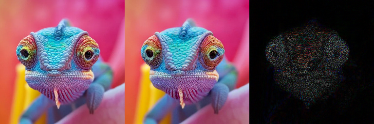
Seems like the compression losses some of the high-frequency information, but otherwise it's a pretty good job.

The diffusion process and the scheduler

The diffusion process starts from gaussian noise. In our case, the noise exists in the latent space, so we initialize the latents which are in the shape of (4, 32, 32).

gen = torch.random.manual_seed(42)
latents = torch.randn(4, 4, 64, 64, generator=gen)

What is this scheduler? sadly this is a bit confusing, so let's try to break it down. Theoretically, what the diffusion model learns is to "reverse" a diffusion process defined as

where \(x^{(0)}\) is a clean normal image, \(\varepsilon\) is standard gaussian noise, and \(\beta_t\) is a coefficient that determines the strength of the "noising" at time step \(t\). Mathematically, if the betas are small enough and the amount of steps taken \(T\) is large enough then \(x^{(T)}\sim\mathcal{N}(0, 1)\). This process is also known as the "forward process". If we knew the noise added, we could "reverse" the process by calculating

And that's the task of the network: given \(x^{(t)}/\sqrt{1-\beta_t}\), it predicts the noise sample added \(\varepsilon\).

Comment: looking into the scheduler a bit more, I see this goes much deeper than I thought (ode derivatives and stuff), so this explanation is probably wrong. I hope to catch up on this eventually, but for now let's get back to the practicalities.

First we initialize the U-Net which is the model that actually predicts the noise.

from diffusers import UNet2DConditionModel
unet = UNet2DConditionModel.from_pretrained("CompVis/stable-diffusion-v1-4", subfolder="unet", torch_dtype=torch.float16).to("cuda")

Before we move on to the inference loop, there's one last detail: in order to steer the model to generate the image according to our prompt, it's not enough to feed in the prompt. We actually feed in two prompts, our own and an empty prompt. We then combine the noise prediction for the empty prompt and the desired prompt in a way that guides the model. We'll see how it's done now

height = 512
width = 512
num_inference_steps = 70
guidance_scale = 7.5

scheduler = LMSDiscreteScheduler(beta_start=0.00085, beta_end=0.012, beta_schedule="scaled_linear", num_train_timesteps=1000)
scheduler.set_timesteps(num_inference_steps)

# initialize the latents as standard normal distribution
gen = torch.random.manual_seed(44)
latents = torch.randn(batch_size, 4, height // 8, width // 8, generator=gen).half().cuda()
latents = latents * scheduler.init_noise_sigma # scale the latents to the initial noise value

for i, t in tqdm(enumerate(scheduler.timesteps)):
    input = torch.cat([latents] * 2)
    input = scheduler.scale_model_input(input, t)

    # predict the noise residual
    with torch.no_grad(): 
        pred = unet(input, t, encoder_hidden_states=text_embeddings).sample

    # perform guidance
    pred_uncond, pred_text = pred.chunk(2)
    pred = pred_uncond + guidance_scale * (pred_text - pred_uncond)

    # compute the "previous" noisy sample
    latents = scheduler.step(pred, t, latents).prev_sample

Running this for a prompt like "A wild pokemon appears!" generates

Wrapping up, if you ended up reading this, I recommend to look at the lecture or at least the notebooks, where you can find an actual working implementation and not just snippets.